Hi, I am Yadokoro from Eukarya.

This is the second in the series of articles on 3D graphics compression techniques, and it will be about the ranged Asymmetric Numerical System.

The ranged Asymmetric Numerical System, or rANS, is a type of entropy codec — a compression algorithm that compresses strings using the probability distribution of their symbols.

Compared to other entropy codecs, rANS is known for its speed and compression ratio: it matches the speed of Huffman coding while providing guaranteed optimality for a given probability distribution.

Polish computer scientist J. Duda introduced the algorithm in 2013 as part of a series of papers on a new family of entropy codecs called asymmetric numerical systems.

The rANS codec quickly became one of the most widely used compression algorithms due to its mathematically guaranteed optimality in compression ratio and computational efficiency.

In fact, it's used by

1. Draco (3D mesh codec by Google)
2. JPEG XL, AV1 (image/video codec)
3. Opus (audio codec)
4. Zstd and LZFSE (general compression algorithms by Meta and Apple, respectively)

…to name a few.

It is also known to be embedded in fundamental systems like operating systems and browsers. Yes, rANS is much more widely used than you might think — even now, as you read this article, an rANS coder is likely at work behind the screen of your device!

Although rANS is a general compression technique rather than a 3D model compression technique, we're including it in our journey through 3D model compression algorithms because these algorithms often make heavy use of rANS codecs.

For example, in the first article of the series, we looked at the Edgebreaker algorithm — an algorithm that converts mesh connectivity into a string of symbols. Since rANS can compress strings, we can feed the resulting string to an rANS coder to achieve a better compression ratio.

Moreover, rANS can also compress attribute values such as vertex coordinates and texture coordinates.

In this article, we will cover the fundamentals of the rANS algorithm.

💡 At Eukarya, we're developing draco-oxide, a Rust rewrite of Google's Draco 3D model compression library. Check it out if you're interested!

The rANS Algorithm

Settings and Notations

Suppose for a finite set $S$ of alphabets. We fix a strict ordering $<$ of $S$.

We may know the probability distribution $p: S \to [0,1]$ of these alphabets so that $\sum_{s \in S} p(s)=1$.

Now for a fixed positive integer $M$, we come up with the discretized probability distribution $P:S \to \N$ in the sense that $\sum_{s \in S} P(s) = M$ and $P(s) \sim p(s)M$ for each $s \in S$.

Furthermore, let $C(s) = \sum_{t\in S:t < s} P(t)$. We call $C(s)$ the offset to the range of $s$.

Encoding

Now we present the encoding formula. Suppose we want to encode a sequence $(s_1, s_2, \cdots, s_m)$ of symbols from $S$, where $m$ is the sequence length.

We set the initial state $X_0=0$. Then rANS recursively computes the state values $(X_1, X_2, \cdots, X_m)$, and the final integer $X_m$ will be our encoded data.

Here's how each recursive step works: Let $E:\Z\times S \to \Z$ denote the function representing the encoding step, so that the encoding step can be written as $X_i = E(X_{i-1},s_i)$ for each time step $i \in \{1,\cdots, m\}$.

We occasionally write $X_i = E_s(X_{i-1})$ when $s\in S$ is fixed.

First, compute the quotient $q$ and remainder $r$ from the Euclidean division of $X_{i-1}$ by $P(s_i)$. That is, find positive integers $q$ and $r<P(s_i)$ such that

$$\begin{align} X_{i-1} = P(s_i) q + r. \end{align}$$

Then $X_i$ is computed by the formula:

$$\begin{align} X_i = E(X_{i-1},s) = q M + C(s_i) + r \end{align}$$

The value $q$ represents a compressed version of the previous state $X_{i-1}$.

When integers are represented in the $M$-ary (or $M$-decimal) number system, multiplying by $M$ shifts each digit one place to the left and inserts a zero in the least significant position, thereby creating space to encode another integer from the set $\{0,\dots,M-1\}$ — this is where the range information is encoded.

We first encode the offset $C(s_i)$ to specify which range we're using, then encode the value $r$, which is guaranteed to lie within the range since $r < P(s_i)$.

The total range information $C(s_i) + r$ is also bounded above by $M$ due to the design of the ranges.

Decoding

Now we give the formula for the decompression algorithm. Decoding a rANS-encoded data involves reversing the encoding process, that is, the symbol that is encoded at last will be decoded first.

Given the state value $X_i$ after encoding $i$ symbols, we need to recover $s_i$ and then compute $X_{i-1}$.

Similarly to the case of encoding, we denote by $D:\Z\to\Z\times S$ the decoding function, i.e., $D(X_i) = (X_{i-1},s_i)$ for each time step $i\in\{1,\cdots,m\}$.

We will first compute the Euclidean division of $X_i$ by $M$, that is, we compute positive integers $Q$ and $R<M$ such that

$$X_i = M Q + R.$$

Since $R$ is a positive integer less than $M$, there must be a unique symbol $s_i\in S$ whose range contains $R$, that is,

$$s_{i} = \max \left\{s : C(s) \leq R \right \}$$

This can be efficiently implemented using a lookup table that maps each value in $\{0,1,\cdots,M-1\}$ to a symbol whose range contains it.

Once we have identified $s_i$, we can compute $X_{i-1}$ by reversing the encoding operation. Note that we have the equations

$$\begin{align} R &= C(s_i)+r \\ Q &= q \end{align}$$

where $q$ and $r$ are the values defined in the encoding function $E$ in the previous section.

Rewriting the variables $q$ and $r$ from equation (1) using equations (3) and (4) gives the final decoding formula:

$$X_{i-1} = P(s_i)Q + R - C(s_i).$$

The decoding process continues recursively until all symbols until we hit $X_i = 0$.

Note that decoding proceeds in reverse order compared to encoding. If we encoded $(s_1, s_2, ..., s_m)$ in this order, then the symbols are decoded in the order $(s_m,s_{m-1},\cdots,s_1)$.

Example

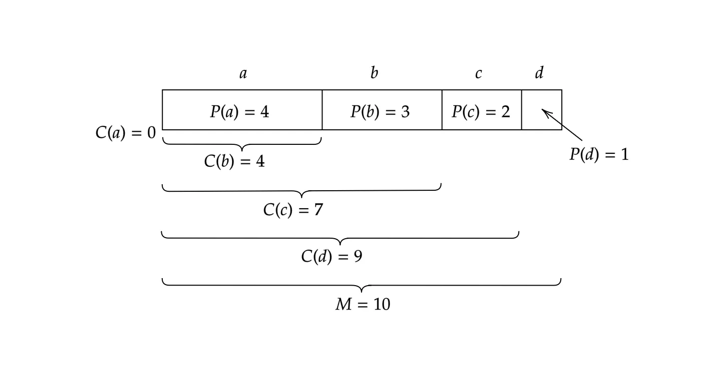
Let’s do a quick example. Suppose that we have the setting of Figure 1 and that we have encoded up to $X_{5}=691$.

Our job now is to encode the 6th symbol, say, “c”. Following the arithmetic, we see that $P(c) = 2$, $q = 345$, $r= 1$, so we obtain $X_6=qM+C(c)+r=3458$.

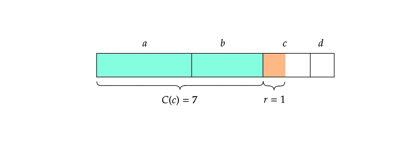
Fine, but how can we decode the state $X_5$ and the symbol “c” back from $X_6$?

Since $C(c)+r$ is less than $M$, dividing $X_6$ by $M$ will give the quotient $Q=q=345$ and the remainder $R=8$.

To decode the symbol and the remainder $r$ from $R$, see Figure 2. Because $C(c) \leq R < C(d)$ (concretely, $7\leq 8 < 9$), we know that $R$ lies in the range of the symbol “$c$”. Also, we see that $R$ has value $1$ in the range of “c”, so we figure out $r=1$.

Thus we obtain $X_{5}=P(c) q + r=691$.

The Streaming rANS Algorithm

The previous section introduced the rANS codec, whose main idea is to create a single large integer containing all information about the string.

While the rANS coder achieves optimal entropy coding for a given probability distribution, it quickly becomes impractical as string size increases — we must perform Euclidean division on increasingly large integers, which is computationally expensive.

To resolve this issue, we decompose each resulting integer $X_i$ to keep it reasonably small.

This is accomplished by the streaming variant of the algorithm, called the streaming rANS algorithm, which we introduce in this section.

Here's how the streaming rANS coder works:

Streaming Encoding

We choose positive integers $k$ and $l$.

The number $k$ indicates how many bits each transfer sends in the stream — set this to $1$ for the simplest implementation, or to $8$ for a byte-stream.

The number $l$ is an algorithm parameter; a higher value of $l$ makes the algorithm slower but improves compression efficiency.

In this section, we will present a streaming variant where, at each time step, the state value lies between $lM$ and $2^k lM-1$, i.e., we make sure that $X_i \in I$ with:

$$I=\{lM,\cdots,2^k l M-1\}.$$

To keep the state value inside $I$ at each time step, we simply divide the state value $X_{i-1}$ by $2^k$ whenever $E(X_{i-1},s)$ would go out of range $I$.

Ok, but how can we know when the state value is about to overflow? Said another way, what state value $X$ and a symbol $s \in S$ will be such that $E(X,s) \in I$?

To answer this question, we need to know what the set $I_s$ defined by

$$I_s=E_s^{-1}(I)$$

looks like.

One fact useful to compute this set is that the function $E_s$ is monotonically increasing, that is, as the input gets bigger and bigger, so does the output.

Indeed, the two numbers $L_s$ and $H_s$ with $L_s = \min \{L: E_s(L)\geq lM \}$ and $H_s = \max\{H:E_s(H)\leq2^klM-1\}$ are all we need to know, as the monotonicity will tell us that any number $X$ with $L_s \leq X \leq H_s$ will be in $I_s$ as well.

So what are the values of $L_s$ and $H_s$? This is in fact a great exercise; if you have extra time, I recommend you close the article now and try to find the answers by yourself.

…welcome back! We should have now arrived at

$$I_s=\{L_s,\cdots, H_s\} = \{lP(s),\cdots,2^k lP(s)-1\}.$$

This clean formula for $I_s$ is in fact thanks to the design of $I$! Thus we now know that if the state value is inside $I_s$ when trying to encode $s$, then the resulting state value $X_i$ would never overflow.

We are finally ready to explain the algorithm. Given the state $X_{i-1}$, a symbol $s_i$ can be encoded by

$$\begin{align} &\text{while } X_{i-1} \not \in I_{s_i} : \\ &\;\;\;\;\text{output } X_{i-1} \mod 2^k \\ &\;\;\;\;X_{i-1} \leftarrow \lfloor X_{i-1} / 2^k \rfloor \\ &X_i = E(s_i,X_{i-1}) \end{align}$$

One question that remains is: how can we be sure that the while loop terminates in a finite step? Isn’t there a case that division by $2^k$ overshoots the $I_{s_i}$?

Well, the division by $2^k$ indeed never overshoots the interval $I_{s_i}$, thanks to the design of $I$.

If there is a state value that overshoots the interval $I_{s_i}$, then there must be an integer $X$ with $I_{s_i}\subsetneq\{X,\cdots,2^kX\}$.

This means that $X \leq lP(s_i)$ and $X > lP(s_i)$, or that $X < lP(s_i)$ and $X \geq lP(s_i)$, but either case can never happen.

Streaming Decoding

For decoding, we perform the reverse operations. We start with the last encoded state $X_m$.

At each time step $i\in\{1,\cdots,m\}$, we start by decoding a symbol $s_i$ and $X_{i-1}$ from $X_i$ using the standard rANS decoding process explained in the previous section.

After decoding a symbol, if the state $X_{i-1}$ falls below the lower bound $kM$ of $I$, we need to read in additional $k$-bits from the encoded bitstream:

$$\begin{align} &(X_{i-1},s) = D(X_i)\\ &\text{while } X_{i-1} < kM: \\ &\;\;\;\;X_{i-1} \leftarrow X_{i-1} \cdot 2^n + \text{next $k$ bits from bitstream} \end{align}$$

You may be wondering whether the number of $k$-bit transfers made during encoding might differ from that during decoding, causing the decoding to fail.

That is, we stop reading the $k$-bit transfers once $X_i \in I$, but isn’t it too early? — isn’t it possible that $2^kX_i\in I$ as well?

Well, once again, the design of $I$ guarantees that there is no integer $X$ such that both $X$ and $2^k X$ are in $I$.

This in turn guarantees that the number of transfers is uniquely determined, so the algorithm does not encounter the ambiguous situation described above.

That is all! We now have a practical rANS algorithm.

Introduction to tANS Algorithm

In this section, we will take a peek at another variant from the ANS family that is closely related to rANS.

In the previous section, we saw the streaming variant of the rANS coder, which limits the state value $X_i$ to a certain range at each time step $i$.

Since $E(X,s)$ is a one-to-one mapping, it means only a finite number of inputs are fed to $E(X,s)$ throughout the entire rANS encoding process.

More specifically, in the streaming variant of rANS, it is sufficient to define $E(X,s)$ for $s \in S$ and $X \in \{lP(s),\cdots,2^klP(s)-1\}$ — there are only finitely many such pairs $(X,s)$.

The tANS algorithm (short for tabled Asymmetric Numerical System) is yet another variant of the ANS algorithm that improves speed by creating a table of $E(X,s)$ at the beginning of the encoding/decoding process.

The table reduces the computations of $E(X,s)$, which include Euclidean divisions and integer multiplications, to a single table lookup.

The challenge lies in the table creation step. We could compute all values of $E(X,s)$, but this would defeat the purpose of tANS, which aims to avoid these computations.

Jarek Duda's paper [1] presents a method for creating a table for $E(X,s)$ without explicitly computing it, but it is way beyond the scope of this article, so let us stop here for this article.

Conclusion

In this article, we've explored the rANS (ranged Asymmetric Numerical System) algorithm and its streaming variant, which serve as powerful tools for data compression in 3D graphics applications.

We've covered both the theoretical foundations and practical implementations of these algorithms.

The basic rANS coder provides optimal entropy coding based on symbol probabilities, but it faces practical limitations due to the growing size of the state value.

The streaming rANS algorithm elegantly solves this problem by introducing a mechanism to bound the state value, making it computationally efficient while preserving compression effectiveness.

We've also briefly touched on tANS (table-based ANS), another variant of the ANS family that offers different trade-offs between compression ratio and computational complexity.

These entropy coding techniques are crucial in modern 3D model compression pipelines. When combined with other techniques like quantization, prediction, and transform coding, they enable significant reductions in file size while maintaining visual quality.

References

1. Duda, J. (2013). Asymmetric numeral systems: entropy coding combining speed of Huffman coding with compression rate of arithmetic coding. arXiv preprint arXiv:1311.2540. https://arxiv.org/pdf/1311.2540